Estimating the heights of New Yorkers from their scuff marks

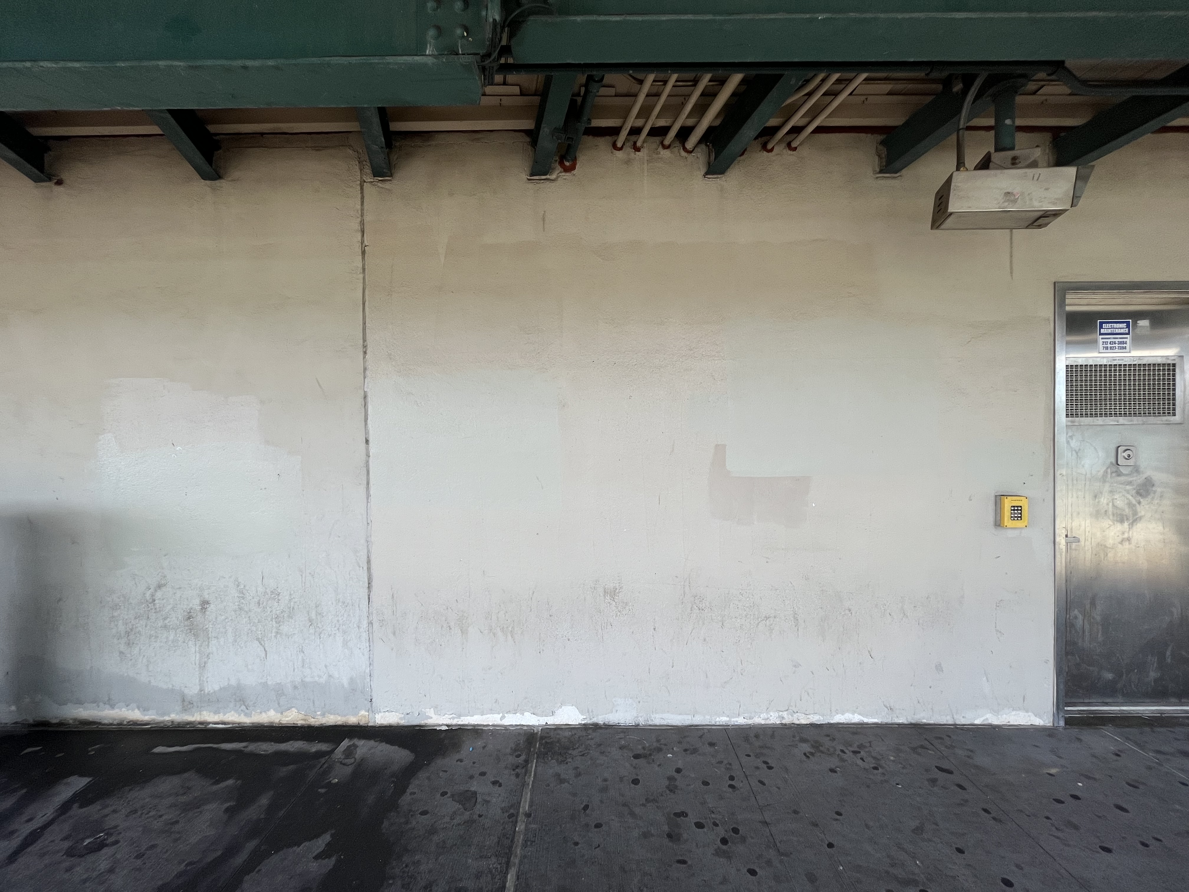
The wall at Smith–Ninth Streets in Brooklyn is made of concrete. Its rough surface holds onto memories longer than the smooth tile that adorns most other stations in the city. A commuter waiting for the train leans with one foot against the wall, and their shoe leaves a mark. It joins marks left by past travelers. In aggregate, they form a darkened band about 18 inches above the floor.

from matplotlib.image import imread
import matplotlib.pyplot as plt
import numpy as np
import cv2

image = imread('IMG_4804.jpg')

IMAGE_WIDTH = image.shape[1]
Y1, Y2, X1, X2 = 1800, 2350, 1300, 3300
GROUND_Y = 2454
KEYPAD_X = 3380
KEYPAD_HEIGHT_PX = 670
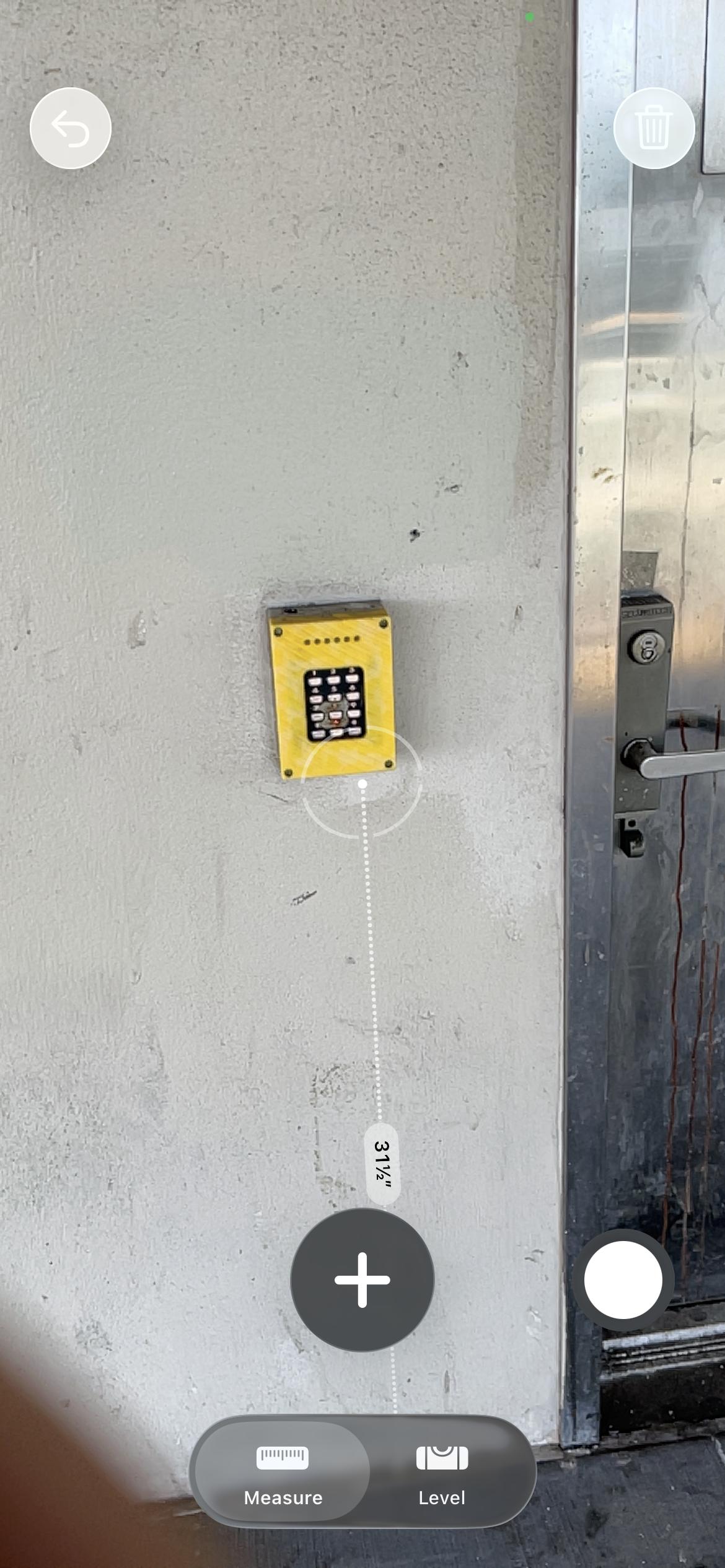
KEYPAD_HEIGHT_IN = 32
PIXELS_PER_INCH = KEYPAD_HEIGHT_PX / KEYPAD_HEIGHT_IN

landmarks = image.copy()
cv2.rectangle(landmarks, (X1, Y1), (X2, Y2), (255, 0, 0), 20)
cv2.line(landmarks, (0, GROUND_Y), (IMAGE_WIDTH, GROUND_Y), (0, 255, 0), 20)
cv2.line(landmarks, (KEYPAD_X, GROUND_Y), (KEYPAD_X, GROUND_Y - KEYPAD_HEIGHT_PX), (0, 0, 255), 10)
plt.imshow(landmarks)

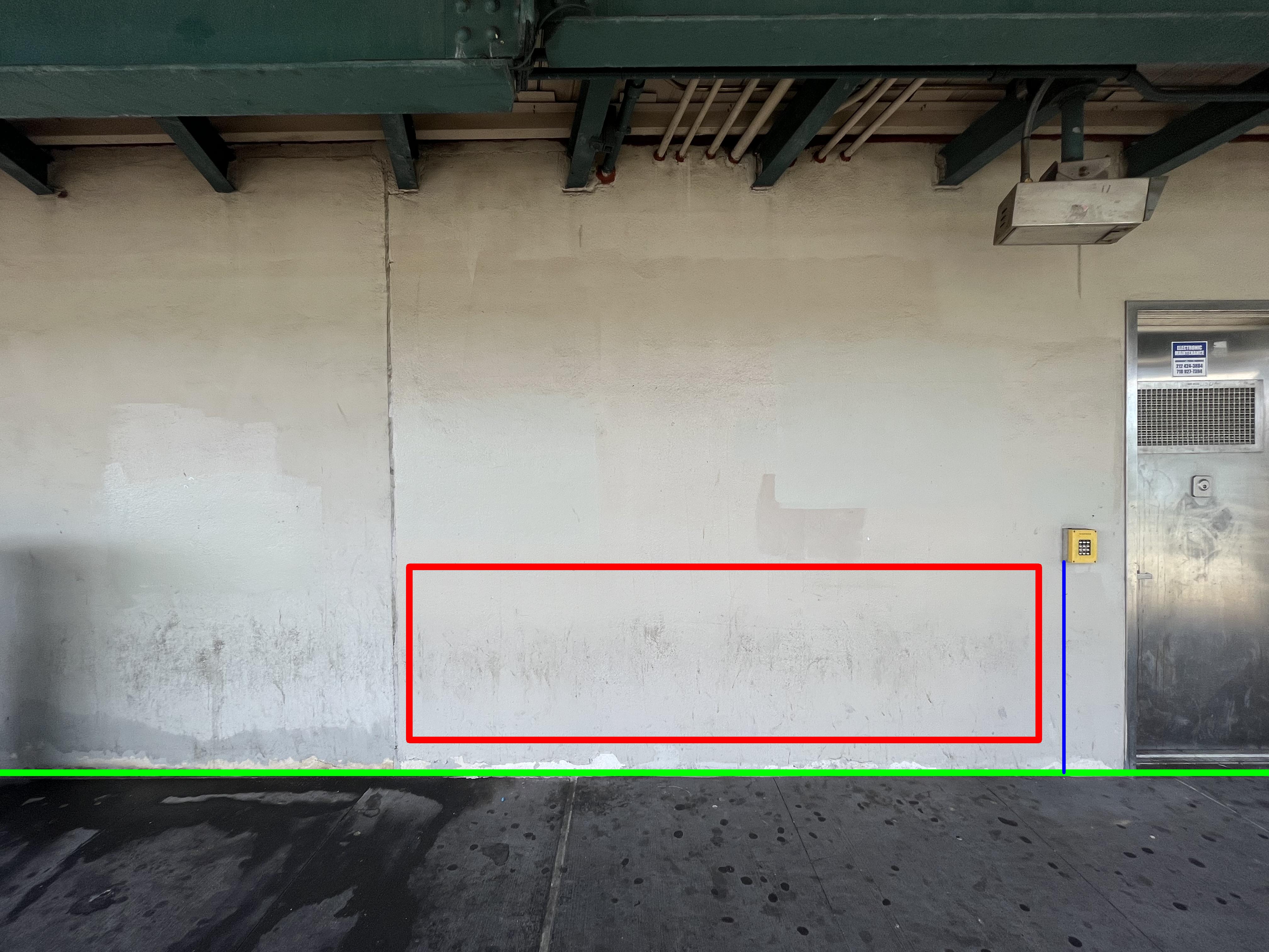
The yellow keypad beside the maintenance door is 32 inches high (I measured it) which gives us a yardstick by which to convert pixel coordinates into physical positions.

Isolating the region with the scuffs, we can compute the relative luminance of each pixel.

region = image[Y1:Y2, X1:X2]
luminance = np.dot(region, [0.2126, 0.7152, 0.0722])
plt.imshow(luminance, cmap='Greys_r')

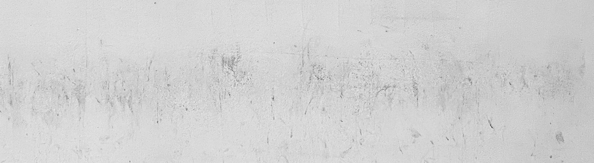
If we take the average of each row, we can plot the darkness of the wall against height from the floor. Darker rows have seen more scuffs.

inches = (GROUND_Y - np.arange(Y1, Y2)) / PIXELS_PER_INCH
avg_luminances = np.mean(luminance, axis=1) / 255
avg_darknesses = 1 - avg_luminances

plt.figure(figsize=(10, 6))
plt.plot(inches, avg_darknesses)

plt.title('Darkness of the wall at Smith–Ninth Streets')
plt.xlabel('Height from ground (inches)')
plt.ylabel('Mean darkness (1 minus relative luminance)')
plt.grid(True, linestyle='--', alpha=0.6)

ticks = np.arange(np.floor(inches.min()), np.ceil(inches.max()))
plt.xticks(ticks[ticks % 2 == 0])

plt.show()

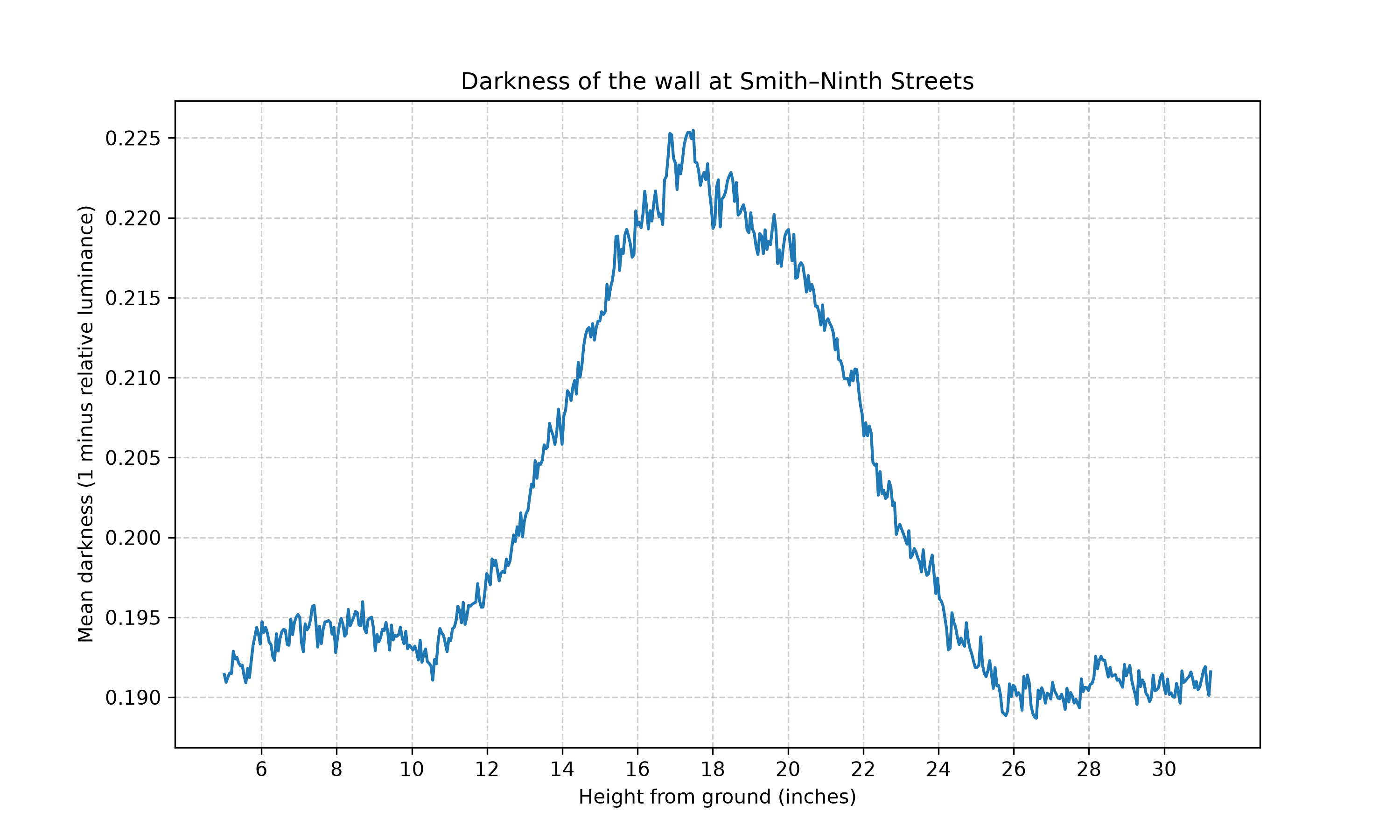
From just a photo, we obtained a distribution of where commuters’ shoes strike the wall. Can we derive how tall they are from this data?

Experimentally, I put my sneakers on and leaned against my bedroom wall, pretending to wait for the F train. The scuff I made landed about 27% up the height of my body. Or, I’m 3.7 times taller than my scuff mark. Assuming this ratio holds for everyone (it doesn’t) we can scale the chart to estimate the heights of the population.

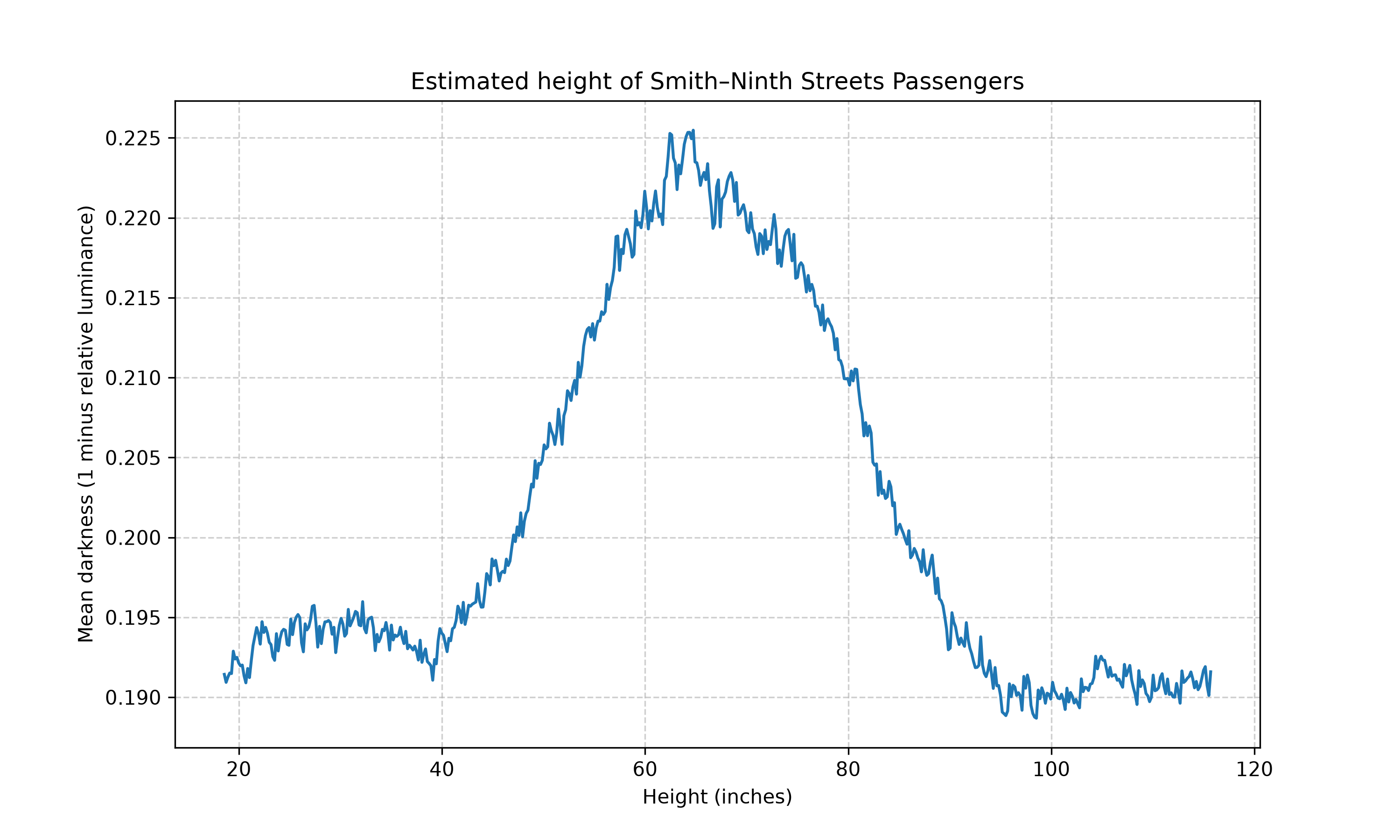
The mean lands on a reasonable spot of five-foot-something, but the variance is too wide. The distribution implies people who are impossibly tall. Besides height, the other variable here is the angle at which people bend their legs: if someone the same height as me kicked their foot up higher, then I’d incorrectly conclude that they’re taller. Our model must account for this.

Future work: if we knew the distribution of angles, then we could do some Bayesian math to correct our estimated height distribution. Send me an email if you want to work together on this! I’d also love to see other cool wear patterns you spot in the wild.